For data engineers and analysts, it’s pretty common to get questions about missing or incorrect data.
“Hey Data Engineer, there’s an issue with the data – I expect numbers at least 20% higher than what our reporting tools show. Can you take a look?”
If you’ve ever been responsible for a Business Intelligence pipeline, you’ve gotten this call. Many, many times. There are a variety of outcomes, listed here in order of increasing difficulty to solve:
- The end-user is incorrect about their intuition, and the data value really is correct
- The end-user wrote a badly formatted query against your data or a query that contained incorrect assumptions
- There’s been a delay in the analytics pipeline
- There’s a bug in the Data Engineering team’s ETL code
- There’s an issue with the source data your BI pipeline is pulling from
The first step is to make sure the problem is not a simple end-user error and that the data is fresh. If it’s neither, you should start debugging your business logic, which is often very painful.
Luckily for us, we are data engineers in a special time. We can take a drastic solution to make sure the question of “how fresh is this data?” never bothers us again:
Every piece of data in your data warehouse or data lake should include a timestamp specifically telling you when that piece of data was last synced from its source of truth.
(Note that we’re not the first people to come up with this idea)
I don’t just mean that you should have a “created” or “updated” timestamp in your main product database – that’s pretty standard practice these days. Instead, I mean that yet another timestamp, while it might seem excessive at first, can save you a lot of time. This timestamp represents the time at which you synced the data from your product database into your data warehouse.
Let’s look at what’s changed to make it worth adding yet another column. The tradeoff here is spending some disk space, in return for answering the “how fresh is this data?” question immediately at debug time.
What Changed?
Data engineering has been around for a long time (over half a century!). Recently, there have been two trends which make our lives easier:
- The cost of data storage has fallen through the floor
- Columnar-based storage engines like AWS Redshift have become more mainstream
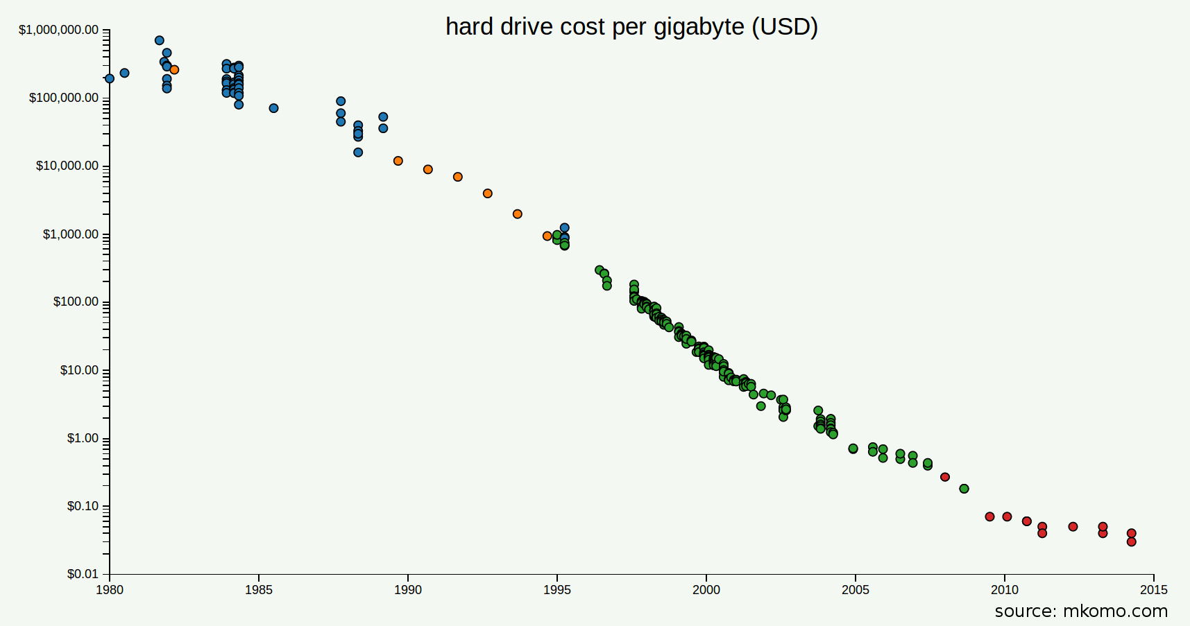
Source: http://www.mkomo.com/cost-per-gigabyte
This changes the math – it’s now cheaper to store timestamp metadata than it is for you to spend time debugging timing errors.
How does it work?
Whenever you have a row in a table, you should have both an “ETL created time”, and if the data can be updated, an “ETL updated time” as well. This is in addition to other timestamps that might already exist in the data.
As an example, imagine we have a “users” table in our product. Whenever we sync a row from that table into our data warehouse, we should update an “_etl_record_timestamp” field, recording when we’ve synced the user over.
Even if this row already has a ‘created’ time corresponding to when the user was created in the product, we should still tag when the BI pipeline synced it. We need the log of when our data warehouse last synced the user, not just when the product initially created or last updated the user.
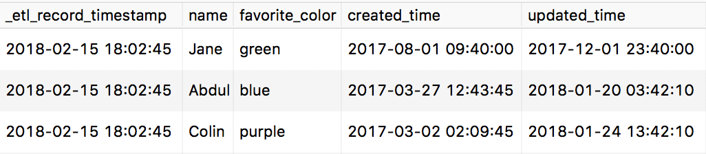
Example table – note that the _etl_record_timestamp is the same for each row.
One decision is whether to set the same timestamp (for instance, when the sync job started running) for all rows, or be even more explicit and set the exact time the job inserted a row. At Clever, we’ve generally gone with just one timestamp as it’s easier to query and reason about, and compresses better. However if your jobs take many minutes or hours, you should revisit this choice.
Clever’s Timestamp Toolkit
We use a few tools to automate snapshotting and adding timestamps. Most of these are OSS, so please use if it makes sense for you!
S3-to-redshift
We created a worker that takes files from Amazon’s s3 service and loads them into Redshift. It uses timestamps as a verification tool. For instance, if we accidentally run a job that would load data into Redshift that’s older than what exists currently, then s3-to-redshift will error. It actually handles timestamps in an even more sophisticated way so that we can support historical views of our data, but more on that in a future blog post…
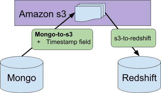
Mongo-to-s3
We use MongoDB for our main product databases. Our data engineering team needs to take that product data and put it into our data warehouse. Mongo-to-s3 takes a config file and performs a snapshot of a MongoDB collection into Amazon’s s3 file storage platform. The worker also flattens JSON objects, filter out sensitive information, and other simple transformations. This data can then be easily loaded into our Amazon Redshift cluster – we use another tool called ‘s3-to-redshift’ to perform this step.
When it pulls from MongoDB, mongo-to-s3 appends a timestamp on each row corresponding to the time when the job began. It’s OSS, so feel free to use this tool for yourself.
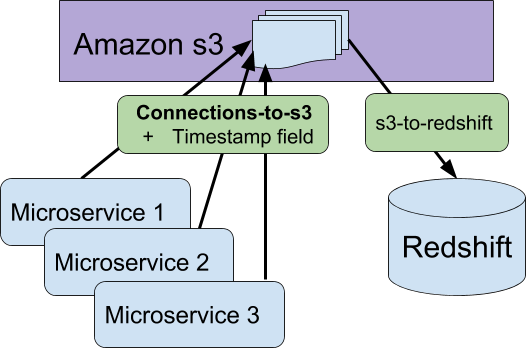
Connections-to-s3
This worker (not OSS) also snapshots our product, but focuses on the “edges” between our different product entities. For instance, if a school in our product is shared with an app, that connection will be snapshotted in a row in the “school-app-connections” table by this worker. It generally tries to use microservices to gain some of the benefits of service isolation. Connections-to-s3 also uploads JSON files of this data to Amazon S3 and also appends a timestamp to each row corresponding to the time the job started.
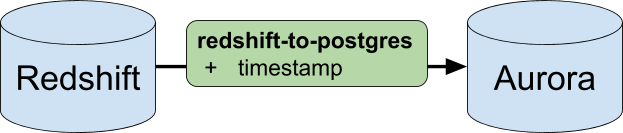
Redshift-to-postgres
We perform business logic calculations in our Redshift cluster, but some queries aren’t as fast as we’d like. So we built redshift-to-postgres (also not OSS) to pull data from our Redshift cluster into our AWS Aurora instance. This worker also sets a timestamp such that we can tell when a piece of data was migrated to Aurora from Redshift.
Analytics-monitor
Finally, once you have this system set up, you start getting further wins. As an example, we have a worker at Clever (analytics-monitor) that checks these timestamps, and lets us know when our BI data has gotten out-of-date beyond a simple threshold. Instead of getting slack messages from the CEO asking why the data is stale, our team is proactively addressing failures and providing a better experience for our internal customers.
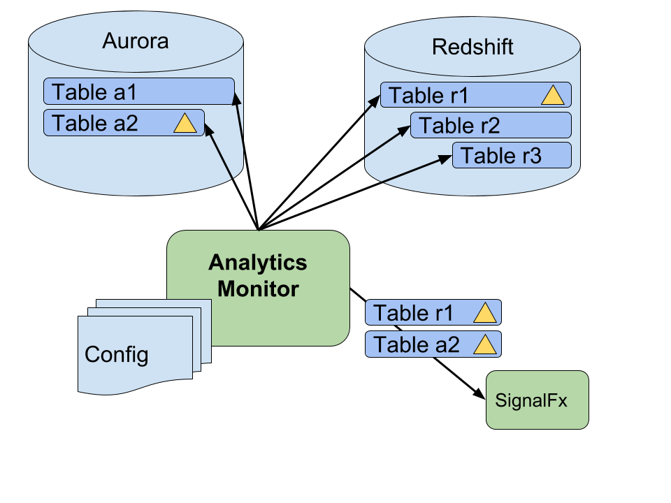
For example, in the above diagram the config for table “r1” might state that it should never be more than 4 hours stale. Analytics-monitor runs and sees that the timestamps in table “r1” are 5 hours old. The worker then triggers an alert via SignalFx for the oncall engineer to take a look at table “r1”.
Costs
If you propose this change, you might get some push-back. “Won’t this cost a lot? It seems wasteful to just store the same item again and again when we can figure this out from our job logs.”
However, the same item over and over again in a column is the best possible case for compression, and since modern data warehouses like Redshift are columnar, it really should only cost a block or two (a fact I’ve verified on Clever’s systems).
Even if you have 100 of these timestamp columns, you’ll end up paying on the order of $1 per year in extra costs.
Example:
One DC2.8xlarge costs $4.80 / hour and contains 2.56TB.
The cost of 100 1MB blocks is:
(100MB / 2.56 TB) * $4.80 * 24 * 365 = $1.64
(this example uses Redshift, using dense compute on-demand instances, which are probably the most expensive).
Then there’s your time. Let’s assume you get 1 “is this data correct” request per week and each request takes you 5 minutes to rule out a BI pipeline latency issue. Over the course of the year, you’ll have spent 4 hours looking into these questions.
(5 minutes * 50 weeks = 4.16 hours)
So the added cost of disk space is worth it, unless you earn 41 cents per hour…! The ROI is positive even if it takes you half a day to implement adding timestamps onto your existing code. Plus, adding the timestamps is way more fun than debugging over the course of the year.
Rejected Alternative
One alternative we thought about: We could just keep a small metadata table containing a row for each table with the latest updates or inserts. Wouldn’t this reduce the redundancy of keeping the same data on each row?
While for non-columnar databases, this might save some disk space, the complexity is simply not worth it. We’d have to keep both tables in sync, and we’d always wonder if the data is really fresh or if there’s a bug in that logic.
We also lose granularity with this solution – for instance we lose the provenance information of a specific piece of data. This could be useful if our ETL pipeline selectively updates data, or if we want to store historical data (more on this in a further blog post).
Lastly since we’re using a columnar database, our compression is optimal for identical data in a column. Thus, we’d get absolutely no material benefit (aka disk / cost savings) from using a separate table.
Conclusion
We live in an era where, for the cost of a sandwich, you could store 24 copies of the “Library of Alexandria” (see comments for calculation). We also live in an era of sophisticated data warehouse technologies.
Instead of spending your time debugging, just spend a bit of disk space and tag your data. You have better things to do, like eating that sandwich. Or, if you want to help evolve how education is used in the classroom, take that time to apply to work at Clever. We’d love to have you help us hack on systems like these.